Estimating $\pi$ using the Monte Carlo Method.
 Image credit: Getty Images
I always asked myself how the scientist have achieved a precise definition for this constant, I guess measuring the circumference with a string and dividing by its diameter is not the easiest way. For this reason in this post I want to show one of the multiples methods to estimate \(\pi\), that using some animations made with ggplot and gganimate.
Introduction
We all know that the symbol used by mathematicians to represent the ratio of a circle’s circumference to its diameter is the lowercase Greek letter \(\pi\).
\[\pi =\frac{C}{d}\]*.](Pi_ratio.svg)
Figure 1: The constant \(\pi\) is defined as the ratio between the circunference to its diamater. Source: Wikipedia.
This ratio is constant, regardless of the circle’s size. pi is perhaps the most famous of the irrational numbers, which means it can not be expressed as a common fraction converting it in an incommensurable number whose digits never settles into a permanently repeating pattern and appear to be randomly distributed.
Nowadays 31 trillon digits of \(\pi\) are known, but do we need really this level of accuracy? NASA indeed has answered this question in a very interesting article I recommend you How Many Decimals of Pi Do We Really Need?.
Monte Carlo method
Monte Carlo methods are a subset of computational algorithms that use the process of repeated random sampling to make numerical estimations of unknown parameters. To estimate \(\pi\) the method consists of drawing on a canvas a square with an inner circle. As we know the area of the circle is \(A_{\bigcirc} = \pi r^2\), and the area of the square is \(A_{\square} = (2r)^2 = 4r^2\), see Figure 2.
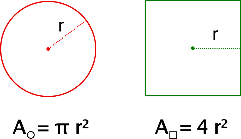
Figure 2: Circle and square areas.
As shown below dividing the area of the circle, by the area of the square we get \(\pi /4\).
\[\frac{A_{\bigcirc}}{A_{\square}} = \frac{\pi \cancel{r^2}}{4 \cancel{r^2}} \Rightarrow \boxed{\pi = 4 \frac{A_{\bigcirc}}{A_{\square}}}\] If a large number of random points inside the square is generated and the quantity of points inside the circle is counted. We can use the following ratio to estimate Pi:
\[ \pi \approx 4 \frac{\text{number of points in the circle}}{\text{total number of points}} \] If you haven’t understand the process yet the following video gives a very clear and didactic explanation about it, this will help you for sure.
Simulations: 1 000 000 million points
To estimate \(\pi\) we are going to plot randomly points using the runif() function and then count how many of them are inside the circle. The canvas in this case is the x-y plane, a square of side 2 units and an inner circle of radius 1 are plotted centered in the origin \((0,0)\). The number of points inside the circle satisfies the condition \(\sqrt{x^{2}+y^{2}} \leq r\), where \(r\) has to be 1 in our case, the radius of the unit circle. The idea now is to estimate \(\pi\) as increasing the number of points, in the code below if the point falls inside the circle was assigned \(1\) otherwise it is \(0\).
In figure 3, \(\pi\) is estimated for 6 different simulations with different sample size to assess how the estimates vary.
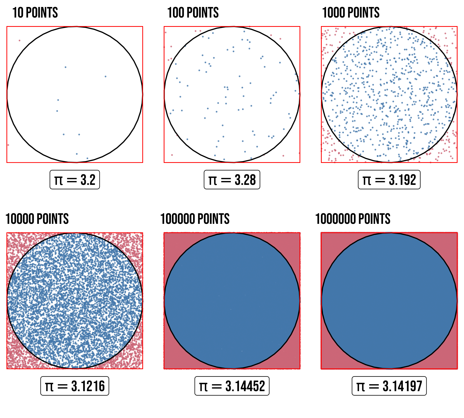
Figure 3: Estimation of \(\pi\) for different point quantities. Points are randomly scattered inside the square, some fall within the unit circle.
Results for some values of \(\pi\) are shown in the Table 1.
| Number of points | Estimation of \(\pi\) |
|---|---|
| 10 | 3.200000 |
| 100 | 3.280000 |
| 1000 | 3.192000 |
| 10000 | 3.121600 |
| 100000 | 3.144520 |
| 1000000 | 3.141972 |
Figure 4 represents the same results shown previously but as an animation, this allow us to understand better the how pi accuracy increases as the sample size do same.
Figure 4: Numerical approximation of \(\pi\).
Figure below show R pi constant value as an horizontal red line. It is seen the convergence to the constant pi is related with the sample size. A sample size of 1,000,000 is used for this simulation.
Figure 5: Estimation of \(\pi\) by sample size. The value is better as the sample points increases.
⚠ NOTE: For the curious people in
Rthe \(\pi\) number is defined by default up to 48 digits.3.141592653589793115997963468544185161590576171875
I hope this short post had been helpful to you. If you have any opinion, suggestion or critic all comments are received, please write me.
Until next time!
Animations code
If you want to reproduce the images and the animations which I used in this post, the complete code can be found here.
Iván Mauricio Cely Toro
PhD student of Physics :flag-br:
100% colombian :flag-co:. Passionate about Science and its teaching. R enthusiast.