 Image credit: Getty Images
One great package in R is the gganimate made by Thomas Lin Pedersen. And just for fun, we are going to explore that. Our aim is to create simple an animated 2D plot representing the relationship between Sine and Cosine.
Packages
Before we begin I show you below the packages employed for the animation.
library(tidyverse) # Easily Install and Load the 'Tidyverse'
library(gganimate) # A Grammar of Animated Graphics
library(hrbrthemes) # Additional Themes, Theme Components and Utilities for 'ggplot2'
As you probably know tidyverse is to manipulate data and to create the visualization and the hrbrthemes package has a very nice set of themes to make our plot visually more pleasant.
Dataset
The first step to elaborate our animation will be to evaluate both trigonometric functions in the angle, for this we will create a data set with a column called theta which is a sequence from \(0\) to \(2\pi\) with 100 elements using the seq() function and then we will calculate the values they take sine and cosine for each angle and we store the results in the columns and, respectively.
df <-
  tibble(theta = seq(0, 2*pi, length.out = 100), ### Angle
         x     = cos(theta), ### x-component
         y     = sin(theta) ### y-component
         )
Recall that in R the arguments of the functions
sin()andcos()are in radians, NOT in degrees.
A quick look at the data allows us to see that when the \(\theta\) is 0, the sine is 0 and the cosine is 1.
| theta | x | y |
|---|---|---|
| 0.0000000 | 1.0000000 | 0.0000000 |
| 0.0634665 | 0.9979867 | 0.0634239 |
| 0.1269330 | 0.9919548 | 0.1265925 |
| 0.1903996 | 0.9819287 | 0.1892512 |
| 0.2538661 | 0.9679487 | 0.2511480 |
| 0.3173326 | 0.9500711 | 0.3120334 |
To appreciate the behavior of each function below, sine and cosine are plotted while \(\theta\) changes.
ggplot(df) +
  geom_line(aes(theta, x, color = "Cosine")) +
  geom_line(aes(theta, y, color = "Sine")) +
  labs(x = "", y = "", color = "") +
  scale_color_manual(values = c("#FAAB18", "steelblue")) +
  coord_fixed() +
  theme_ipsum()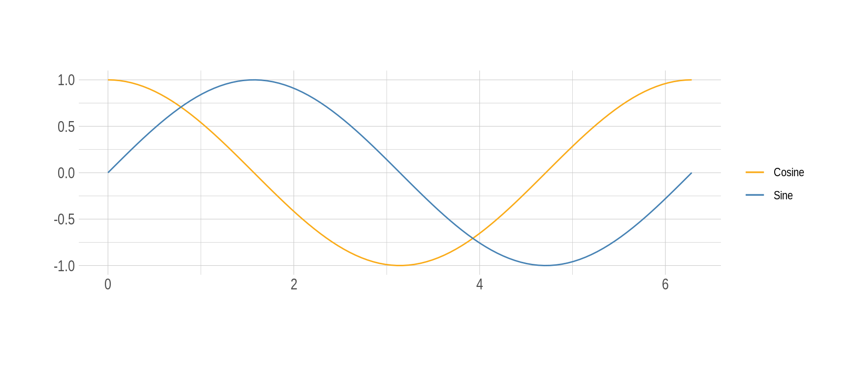
Figure 1: Evolution of sine and cosine functions as \(\theta\) changes
It can be seen that both functions take values between $ -1 $ and $ 1 $, although both oscillate in the same way, it seems that they are displaced horizontally or better out of phase with respect to each other. Being curious we could ask ourselves what happens if we graph the cosine values on the abscissa and those of the sine on the ordinate. Voilà!, we get a circle as a result.
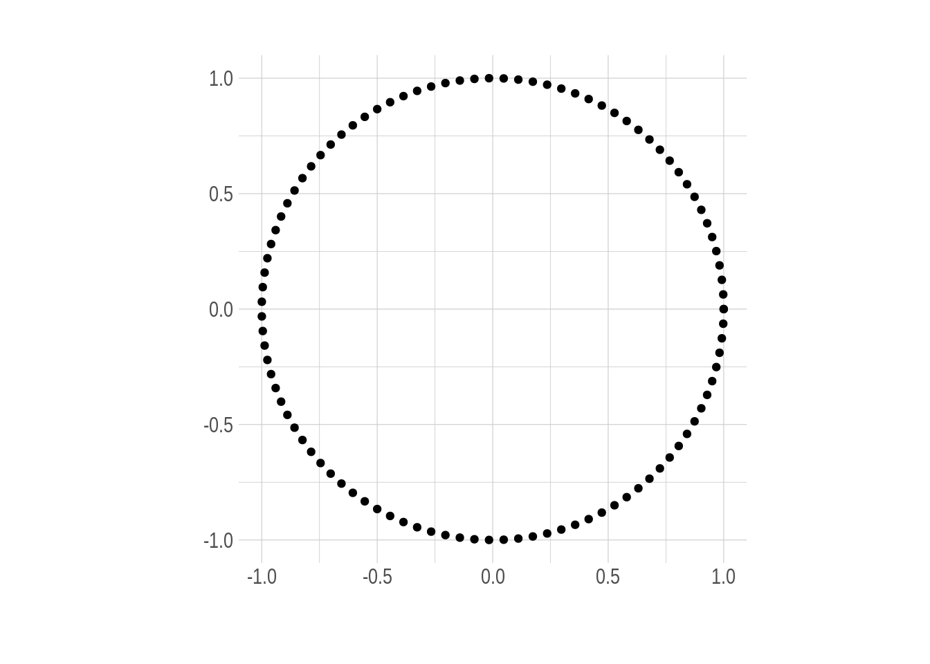
Figure 2: The unit circle
How are the functions Sine and Cosine related to a circle? Let’s find out. This circle is known as the unit circle, which has radius 1 and is centered at the origin \((0,0)\) of the Cartesian coordinate system. The importance of this circle is that it makes some math topics easier and more manageable. In the case of trigonometry for any angle \(\theta\), the values for sine and cosine are nothing more than \(sin(\theta) = y\) and \(cos(\theta) = x\).
Using sine and cosine, it is possible to describe any point \((x,y)\) as an alternative to the point \((r, \theta)\), where \(r\) is the length of a line segment from the origin to the point and \(\theta\) is the angle between the line segment and the x-axis. This is called the polar coordinate system and the relation \((x,y) = \left( rcos(\theta),rsin(\theta) \right)\) is used to convert. If you want to better understand and see how this relationship is, visit this site.
ggplot(df) +
  geom_path(aes(x = x, y= y)) +
  geom_point(aes(x = cos(pi/4), y = sin(pi/4)), color = "red", size = 2) +
  geom_segment(aes(x = 0, y = 0, xend = cos(pi/4), yend = sin(pi/4)),
               arrow = arrow(length = unit(1.7, "mm"))) +
  geom_segment(aes(x = 0, y = sin(pi/4), xend = cos(pi/4), yend = sin(pi/4)),
               color = "#FAAB18") +
  geom_segment(aes(x = cos(pi/4), y = 0, xend = cos(pi/4), yend = sin(pi/4)),
               color = "steelblue") +
  geom_hline(yintercept = 0, linetype = 2) +
  geom_vline(xintercept = 0, linetype = 2) +
  labs(x = "", y = "") +
  coord_fixed() +
  theme_ipsum()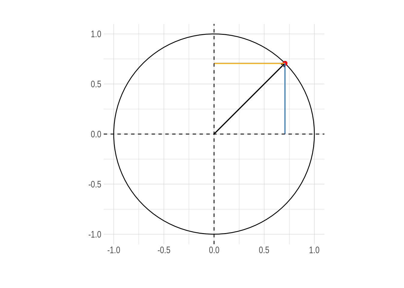
Figure 3: Unit circle. The components of any point \((x,y)\) on the circumference represent the cosine and sine of the angle \(\theta\) that forms with the horizontal respectively.
The task now is to combine the graphs of the circle and the sine and cosine. At the end of the post you will find code that I used to create the animation that you see in Figure 4.
Figure 4: Animation of the relationship between the unit circle, sine and cosine
Starting from the origin, the arrow travels the circumference of radius 1 from the horizontal axis completing a 360 degree turn. Horizontal and vertical components represent trigonometric functions as the angle varies, as seen when one grows the other decreases.
If we take the vertical projection of the point around our circumference and project it in a straight line (along the axis \(y\)) in the plot it is to the right of the circle. This brings us to the red dot. The coordinate \(y\) of this red point is the value of the sine function evaluated at the angle \(\theta\).
- Coordinate of the vertically oscillating point \(y = sin (\theta)\)
As the angle \(\theta\) changes, we can see the red dot move up and down, tracing the blue graph. This is the graph for the sine function. The dashed lines you see passing mark each quadrant along the circle, that is, at each angle of $ 90° $ or \(\pi/2\) radians. Notice how the sine curve goes from 1, to zero, to -1, then returns to zero, exactly on these lines. This reflects the fact that $ sin(0) = 0 $, \(sin(\pi/2) = 1\), \(sin(\pi) = 0\), and \(sin(3 \pi / 2) = -1\) .
If we follow the same reasoning and imagine a projected point parallel to the coordinate \(x\), it is possible to deduce the behavior of the cosine function evaluated at angle \(\theta\), that is:
- Coordinate of the point that oscillates horizontally $ x = cos() $
The yellow curve drawn by this imaginary point is the graph of the cosine function. Look again at how it behaves when it crosses each quadrant, reflecting the fact that \(cos(0) = 1\), \(cos(\pi/2) = 0\), \(cos(\pi) = -1\), and \(cos( 3\pi / 2) = 0\).
Now is your time to try. I hope this animation and short explanation about the unit circle and the sine and cosine function are useful to you. Until next time!
Code:
If you prefer you can find a script with the complete code here.
library(tidyverse) # Easily Install and Load the 'Tidyverse'
library(gganimate) # A Grammar of Animated Graphics
library(hrbrthemes) # Additional Themes, Theme Components and Utilities for 'ggplot2'

df <-
  tibble(theta = seq(0, 2*pi, length.out = 100), ### Angle
         x     = cos(theta), ### x-component
         y     = sin(theta) ### y-component
         )

### Add frame colum for each step of the animation
df <-
df %>%
  mutate(frame = 1:n()) %>%
  relocate(frame)

### Labels superior axis in radians
rad_labels <-  c(expression(phantom(over(1,1))*0*phantom(over(1,1))),
                       expression(frac(pi, 4)),
                       expression(frac(pi, 2)),
                       expression(frac(3*pi, 4)),
                       expression(phantom(over(1,1))*pi*phantom(over(1,1))),
                       expression(frac(5*pi, 4)),
                       expression(frac(3*pi, 2)),
                       expression(frac(7*pi, 4)),
                       expression(phantom(over(1,1))*2*pi*phantom(over(1,1)))
                 )


sine <-
ggplot(df) +
  ### Circle
  geom_point(aes(x, y)) +
  geom_path(aes(x, y)) +
  ### Angle arrow
  geom_segment(aes(x = 0, y = 0, xend = x, yend = y), arrow = arrow(length = unit(1.7, "mm"), type = "closed")) +
  geom_segment(aes(x = 2, y = 0, xend = Inf, yend = 0), linetype = "dashed") +
  ### Red point and its line
  geom_point(aes(x = 1.5, y = y), color = "red", size = 2) +
  geom_vline(xintercept = 2) +
  ### Connecting lines circle and functions
  geom_segment(aes(x = x, y = y, xend = theta + 2, yend = y)) +
  geom_segment(aes(x = 0, y = 0, xend = 0, yend = y), color = "steelblue") +
  geom_segment(aes(x = x, y = 0, xend = x, yend = y), color = "steelblue", linetype = 2) +
  geom_text(aes(x = -0.12, y = 0.5, label = "sin(theta)"), color = "steelblue", parse = T, angle = 90) +
  geom_segment(aes(x = 0, y = 0, xend = x, yend = 0), color = "#FAAB18") +
  geom_segment(aes(x = 0, y = y, xend = x, yend = y), color = "#FAAB18", linetype = 2) +
  geom_text(aes(x = 0.5, y = -0.12, label = "cos(theta)"), color = "#FAAB18", parse = T) +
  geom_path(aes(theta + 2, y), color = "steelblue") +
  geom_point(aes(x = theta + 2, y =  y), color = "steelblue") +
  geom_path(aes(theta + 2, x), color = "#FAAB18") +
  geom_point(aes(x = theta + 2, y =  x), color = "#FAAB18") +
  coord_fixed(expand = F, xlim = c(-1.1, 8.4), ylim = c(-1.1, 1.1)) +
  scale_x_continuous(breaks = c(-1:1, seq(2, (2*pi) + 2, length.out = 9)),
                     labels = c(-1:1, seq(0, 360, length.out = 9)), name = "degrees",
                     sec.axis = sec_axis(trans = ~.*1,
                                         breaks = c(rep(NA,3), seq(2, (2*pi)+2, length.out = 9)),
                                         labels =  c(-1:1, rad_labels),
                                         name =   "radians")) +
  labs(title = "Unit Circle - Sine and Cosine Functions",
       subtitle = "Sine and cosine can be generated by projecting the tip of a vector onto the y-axis and x-axis as the\n vector rotates about the origin.",
       caption = "Created by @Mauricio_Cely",
       y = "") +
  theme_ipsum() +
  theme(plot.margin = margin(-1, 1, -1, 0, unit = "cm"),
        plot.subtitle = element_text(face = "italic")) +
  transition_reveal(along = frame)

# options(gganimate.dev_args = list(res = 115))

animate(sine,
        width = 1600, # 900px wide
        height = 800, # 600px high
        duration = 10,
        renderer = gifski_renderer(),
        res = 200) # 10 frames per second

anim_save("unit_circle.gif")Iván Mauricio Cely Toro
PhD student of Physics :flag-br:
100% colombian :flag-co:. Passionate about Science and its teaching. R enthusiast.